Utilities functions

Use this module for utility functions.

>>> import opticomlib.utils as ut

Functions

dec2bin(num[, digits])	Converts an integer to its binary representation.
str2array(string[, dtype])	Converts a string to array of numbers.
get_time(line_of_code, n)	Get the average time of execution of a line of code.
tic()	Start a timer.
toc()	Stop a timer.
db(x)	Calculates the logarithm in base 10 of the input x and multiplies it by 10.
dbm(x)	Calculates dBm from Watts.
idb(x)	Calculates the number value from a dB value.
idbm(x)	Calculates the power value in Watts from a dBm value.
gaus(x[, mu, std])	Gaussian function.
Q(x)	Q-function.
phase(x[, zero_ref_index])	Calculate the unwrapped phase the signal.
tau_g(x, fs)	Calculate the group delay of a frequency response.
dispersion(x, fs, f0)	Calculate the dispersion of a frequency response.
bode(H, fs[, f0, xaxis, disp, yscale, ret, ...])	Plot the Bode plot of a given transfer function H (magnitude, phase and group delay).
rcos(x, alpha, T)	Raised cosine spectrum function.
si(x[, unit, k])	Unit of measure classifier.
norm(x)	Normalize an array by dividing each element by the maximum value in the array.
nearest(x, a)	Find the value of X closest to a.
theory_BER(P_avg, modulation[, M, decision, ...])	This function calculates the bit error rate (BER) for an OPTICAL RECEIVER, based on a PIN photodetector, from the average input power.
p_ase([amplify, wavelength, G, NF, BW_opt])	Calculate the ASE noise power [Watts].
average_voltages(P_avg, modulation[, M, ER, ...])	Calculate the average voltages of the ON and OFF slots [Voltages].
noise_variances(P_avg, modulation[, M, ER, ...])	Calculate the theoretical noise variances for OFF and ON slots, include sig-ase, ase-ase, thermal and shot noises [V^2].
optimum_threshold(mu0, mu1, S0, S1, modulation)	Calculate the optimum threshold for binary modulation formats.
shortest_int(x[, percent])	Estimation of the shortest interval of x values, containing {percent}% of the samples in 'x'.
eyediagram(y, sps[, n_traces, cmap, ...])	Plots a colored eye diagram, internally calculating color density.
rcos_pulse(beta, span, sps[, shape])	Generate a raised cosine or root raised cosine filter impulse response.
gauss_pulse(span, sps[, T, m, c])	Generate a Gaussian or Super-Gaussian filter.
nrz_pulse(span, sps, T)	Generate a Non-Return-to-Zero (NRZ) pulse shape.
upfir(x, h[, up])	Replicate MATLAB's upfirdn function for upsampling and FIR filtering.
phase_estimator(t, x, f)	Estimates the phase and amplitude of a sinusoid with known frequency.
get_psd(signal, fs[, nperseg])	Calculate the Power Spectral Density (PSD) of a signal using Welch's method.

opticomlib.utils.dec2bin(num: int, digits: int = 8)

Converts an integer to its binary representation.

Parameters:

• num (int) – Integer to convert.

• digits (int, default: 8) – Number of bits of the binary representation.

Returns:

Binary representation of num of length digits.

Return type:

binary_sequence

Raises:

• ValueError – If num is not an integer number.

• ValueError – If num is too large to be represented with digits bits.

Example

>>> dec2bin(5, 4)
array([0, 1, 0, 1], dtype=uint8)

opticomlib.utils.str2array(string: str, dtype: bool | int | float | complex | None = None)

Converts a string to array of numbers. Use comma (,) or whitespace (`` ) as element separators and semicolon (;``) as row separator. Also, i or j can be used to represent the imaginary unit.

Parameters:

• string (str) – String to convert.

• dtype (type, optional) – Data type of the output array. If dtype is not given, the data type is determined from the input string. If dtype is given, the data output is cast to the given type. Allowed values are bool, int, float and complex.

Returns:

arr – Numeric array.

Return type:

np.ndarray

Raises:

ValueError – If the string contains invalid characters.

Example

For binary numbers, string must contain only 0 and 1. Only in this case, sequence don’t need to be separated by commas or spaces although it is allowed.

>>> str2array('101')
array([ True, False, True])
>>> str2array('1 0 1; 0 1 0')
array([[ True, False,  True],
       [False,  True, False]])

Special case >>> str2array(‘1 0 1 10’) array([True, False, True, True, False]) >>> str2array(‘1 0 1 10’, dtype=int) array([ 1, 0, 1, 10]) >>> str2array(‘1 0 1 10’, dtype=float) array([ 1., 0., 1., 10.]) >>> str2array(‘1 0 1 10’, dtype=complex) array([ 1.+0.j, 0.+0.j, 1.+0.j, 10.+0.j])

For integer and float numbers >>> str2array(‘1 2 3 4’) array([1, 2, 3, 4]) >>> str2array(‘1.1 2.2 3.3 4.4’) array([1.1, 2.2, 3.3, 4.4])

For complex numbers >>> str2array(‘1+2j 3-4i’) array([1.+2.j, 3.-4.j])

opticomlib.utils.get_time(line_of_code: str, n: int)

Get the average time of execution of a line of code.

Parameters:

• line_of_code (str) – Line of code to execute.

• n (int) – Number of iterations.

Returns:

time – Average time of execution, in seconds.

Return type:

float

Example

>>> get_time('for i in range(1000): pass', 1000)
1.1955300000010993e-05

opticomlib.utils.tic()

Start a timer. Create a global variable with the current time. Then you can use toc() to get the elapsed time.

Example

>>> tic() # wait some time
>>> toc()
2.687533378601074

opticomlib.utils.toc()

Stop a timer. Get the elapsed time since the last call to tic().

Returns:

time – Elapsed time, in seconds.

Return type:

float

Example

>>> tic() # wait some time
>>> toc()
2.687533378601074

opticomlib.utils.db(x)

Calculates the logarithm in base 10 of the input x and multiplies it by 10.

\[\text{db} = 10\log_{10}{x}\]

Parameters:

x (Number or Array_Like) – Input value (x>=0).

Returns:

out – dB value.

Return type:

float or np.ndarray

Raises:

• TypeError – If x is not a number, list, tuple or ndarray.

• ValueError – If x or any(x) < 0.

Example

>>> db(1)
0.0
>>> db([1,2,3,4])
array([0.        , 3.01029996, 4.77121255, 6.02059991])

opticomlib.utils.dbm(x)

Calculates dBm from Watts.

\[\text{dbm} = 10\log_{10}{x}+30\]

Parameters:

x (Number or Array_Like) – Input value (x>=0).

Returns:

out – dBm value. If x is a number, then the output is a float. If x is an array_like, then the output is an np.ndarray.

Return type:

float or np.ndarray

Raises:

• TypeError – If x is not a number, list, tuple or ndarray.

• ValueError – If x or any(x) < 0.

Example

>>> dbm(1)
30.0
>>> dbm([1,2,3,4])
array([30.        , 33.01029996, 34.77121255, 36.02059991])

opticomlib.utils.idb(x)

Calculates the number value from a dB value.

\[y = 10^{\frac{x}{10}}\]

Parameters:

x (Number or Array_Like) – Input value.

Returns:

out – Number value. If x is a number, then the output is a float. If x is an array_like, then the output is an np.ndarray.

Return type:

float or np.ndarray

Example

>>> idb(3)
1.9952623149688795
>>> idb([0,3,6,9])
array([1.        , 1.99526231, 3.98107171, 7.94328235])

opticomlib.utils.idbm(x)

Calculates the power value in Watts from a dBm value.

\[y = 10^{(\frac{x}{10}-3)}\]

Parameters:

x (Number or Array_Like) – Input value.

Returns:

out – Power value in Watts. If x is a number, then the output is a float. If x is an array_like, then the output is an np.ndarray.

Return type:

float or np.ndarray

Example

>>> idbm(0)
0.001
>>> idbm([0,3,6,9])
array([0.001     , 0.00199526, 0.00398107, 0.00794328])

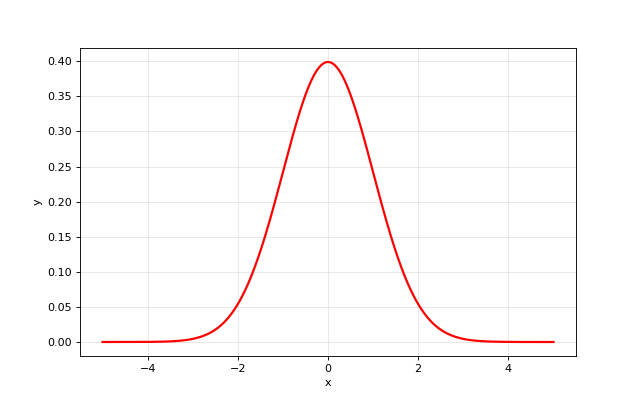
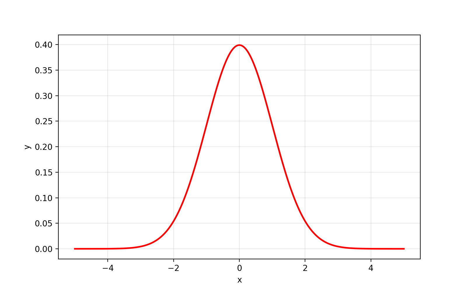
opticomlib.utils.gaus(x, mu: float = None, std: float = None)

Gaussian function.

\[\text{gaus}(x) = \frac{1}{\sigma\sqrt{2\pi}}e^{-\frac{(x-\mu)^2}{2\sigma^2}}\]

Parameters:

• x (Number or Array_Like) – Input value.

• mu (float, default: 0) – Mean.

• std (float, default: 1) – Standard deviation.

Returns:

out – Gaussian function value. If x is a number, then the output is a float. If x is an array_like, then the output is an np.ndarray.

Return type:

float or np.ndarray

Examples

>>> gaus(0, 0, 1)
0.3989422804014327
>>> gaus([0,1,2,3], 0, 1)
array([0.39894228, 0.24197072, 0.05399097, 0.00443185])

from opticomlib import gaus
import matplotlib.pyplot as plt
import numpy as np

x = np.linspace(-5, 5, 1000)
y = gaus(x, 0, 1)

plt.figure(figsize=(8, 5))
plt.plot(x, y, 'r', lw=2)
plt.ylabel('y')
plt.xlabel('x')
plt.grid(alpha=0.3)
plt.show()

(Source code, png, hires.png, pdf)

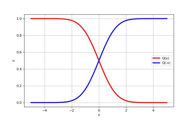
opticomlib.utils.Q(x)

Q-function.

\[Q(x) = \frac{1}{2}\text{erfc}\left( \frac{x}{\sqrt{2}} \right)\]

Parameters:

x (Numper or Array_Like) – Input value.

Returns:

out – Q(x) values. If x is a number, then the output is a float. If x is an array_like, then the output is an np.ndarray.

Return type:

float or np.ndarray

Examples

>>> Q(0)
0.5
>>> Q([0,1,2,3])
array([0.5       , 0.15865525, 0.02275013, 0.0013499 ])

from opticomlib import Q
import matplotlib.pyplot as plt
import numpy as np

x = np.linspace(-5, 5, 1000)

plt.figure(figsize=(8, 5))
plt.plot(x, Q(x), 'r', lw=3, label='Q(x)')
plt.plot(x, Q(-x), 'b', lw=3, label='Q(-x)')
plt.ylabel('y')
plt.xlabel('x')
plt.legend()
plt.grid()
plt.show()

(Source code, png, hires.png, pdf)

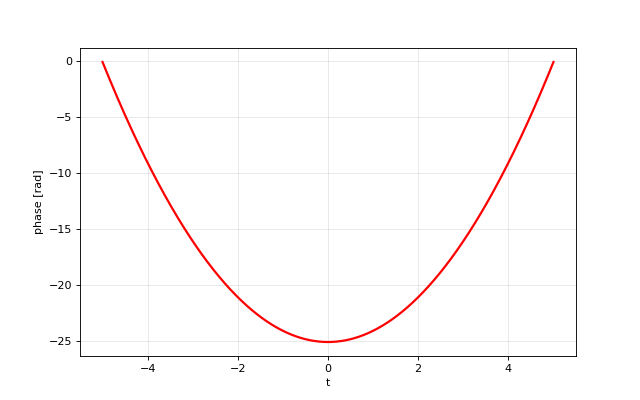
opticomlib.utils.phase(x: ndarray, zero_ref_index: int = None)

Calculate the unwrapped phase the signal.

Parameters:

• x (np.ndarray) – Signal to calculate the phase

• zero_ref_index (int, default: None) – Position of signal to take zero phase reference. By default zero phase reference is set to position 0 of x.

Returns:

phase – Unwrapped phase in radians.

Return type:

np.ndarray

Examples

from opticomlib import phase
import matplotlib.pyplot as plt
import numpy as np

t = np.linspace(-5, 5, 1000)
y = np.exp(1j*t**2)
phi = phase(y)

plt.figure(figsize=(8, 5))
plt.plot(t, phi, 'r', lw=2)
plt.ylabel('phase [rad]')
plt.xlabel('t')
plt.grid(alpha=0.3)
plt.show()

(Source code, png, hires.png, pdf)

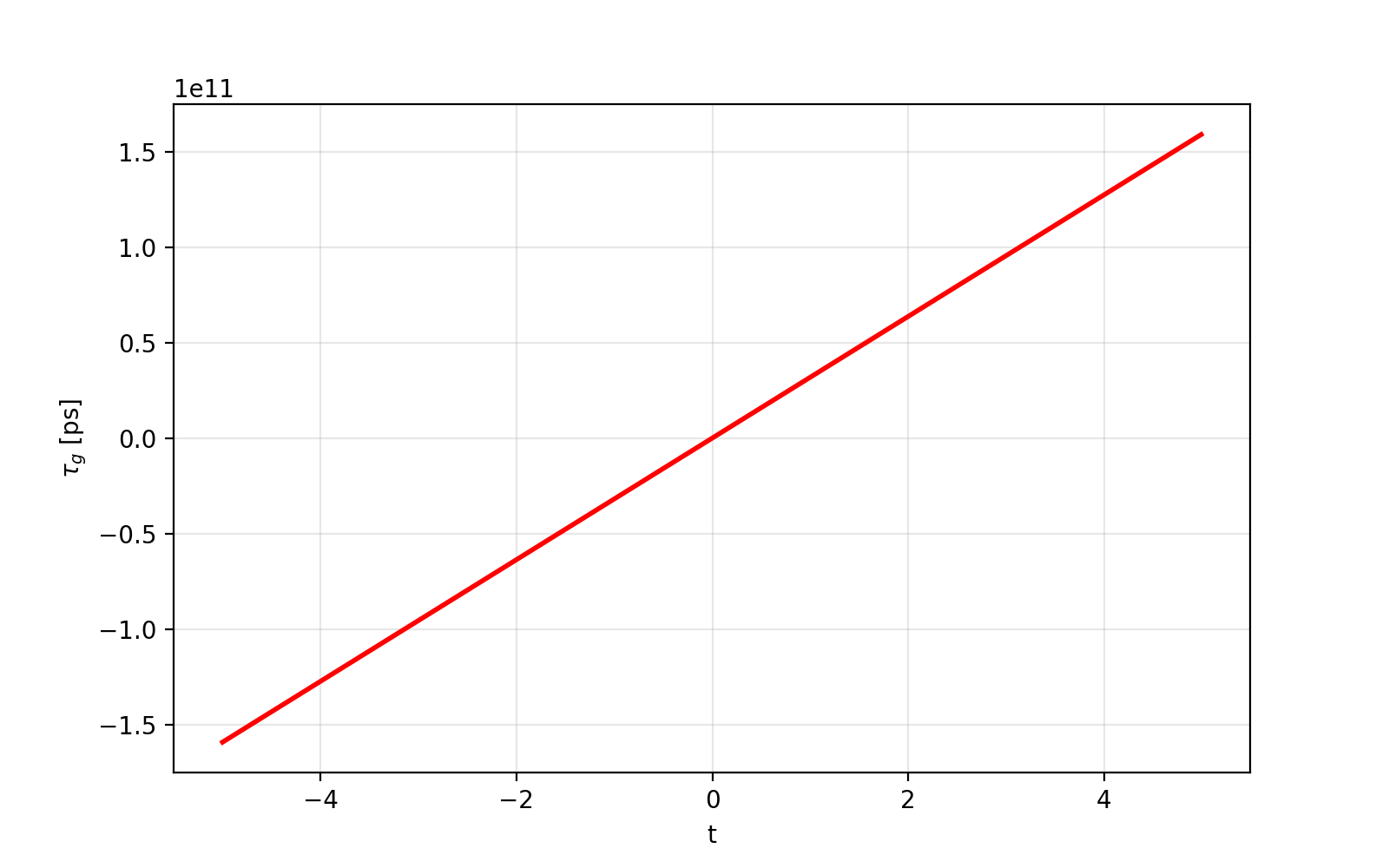
opticomlib.utils.tau_g(x: ndarray, fs: float)

Calculate the group delay of a frequency response.

Parameters:

• x (np.ndarray) – Frequency response of a system.

• fs (float) – Sampling frequency of the system.

Returns:

tau – Group delay of the system, in [ps].

Return type:

np.ndarray

Examples

from opticomlib import tau_g
import matplotlib.pyplot as plt
import numpy as np

t = np.linspace(-5, 5, 1000)
y = np.exp(1j*t**2)
phi = tau_g(y, 1e2)

plt.figure(figsize=(8, 5))
plt.plot(t, phi, 'r', lw=2)
plt.ylabel(r'$\tau_g$ [ps]')
plt.xlabel('t')
plt.grid(alpha=0.3)
plt.show()

(Source code, png, hires.png, pdf)

opticomlib.utils.dispersion(x: ndarray, fs: float, f0: float)

Calculate the dispersion of a frequency response.

Parameters:

• x (np.ndarray) – Frequency response of a system.

• fs (float) – Sampling frequency of the system.

• f0 (float) – Center frequency of the system.

Returns:

D – Cumulative dispersion of the system, in [ps/nm].

Return type:

np.ndarray

opticomlib.utils.bode(H: ndarray, fs: float, f0: float = None, xaxis: Literal['f', 'w', 'lambda'] = 'f', disp: bool = False, yscale: Literal['linear', 'db'] = 'linear', ret: bool = False, retAxes: bool = False, show_: bool = True, xlim: tuple = None)

Plot the Bode plot of a given transfer function H (magnitude, phase and group delay).

Parameters:

• H (np.ndarray) – The transfer function.

• fs (float) – The sampling frequency.

• f0 (float, default: None) – The center frequency. If not None, dispersion are also plotted.

• xaxis (str, default: ‘f’) – The x-axis (frequency, angular velocity, wavelength).

• disp (bool, default: False) – Whether to plot the dispersion.

• ret (bool, default: False) – Whether to return the plotted data.

• show (bool, default: True) – Whether to display the plot.

• style (str, default: ‘dark’) – The plot style.

Returns:

(f, H, phase, tau_g) – A tuple containing the frequency, magnitude, phase, and group delay if ret=True.

Return type:

np.ndarray

Raises:

ValueError – If style is not “dark” or “light”.

Example

>>> from opticomlib import bode
>>> H, phase, tau_g = bode(H, fs, ret=True, show_=False)

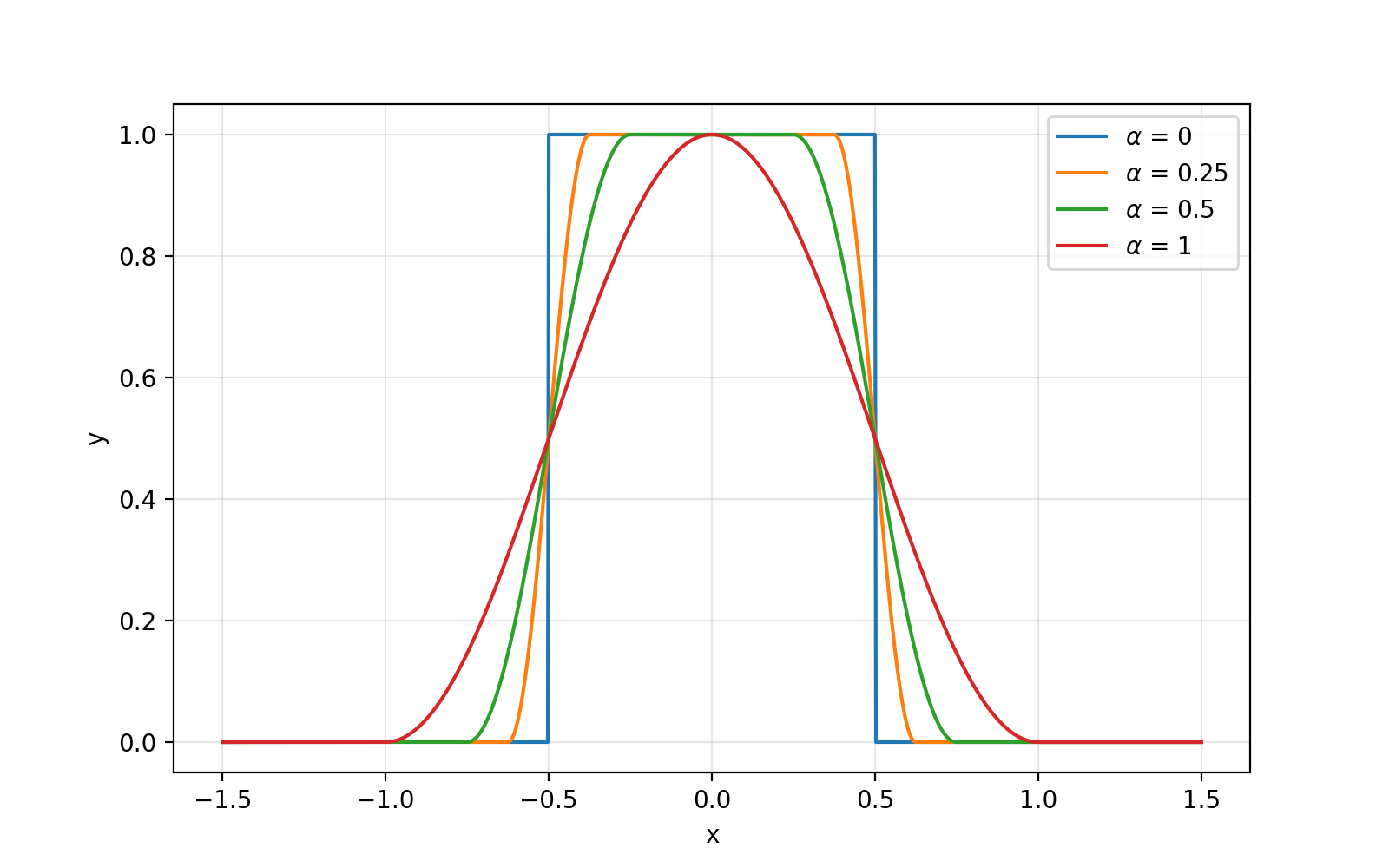
opticomlib.utils.rcos(x, alpha, T)

Raised cosine spectrum function.

Parameters:

• x (Number or Array_Like) – Input values.

• alpha (float) – Roll-off factor.

• T (float) – Symbol period.

Returns:

Raised cosine function.

Return type:

np.ndarray

Example

https://en.wikipedia.org/wiki/Raised-cosine_filter

from opticomlib import rcos
import matplotlib.pyplot as plt
import numpy as np

T = 1
x = np.linspace(-1.5/T, 1.5/T, 1000)

plt.figure(figsize=(8, 5))

for alpha in [0, 0.25, 0.5, 1]:
    plt.plot(x, rcos(x, alpha, T), label=r'$\alpha$ = {}'.format(alpha))

plt.ylabel('y')
plt.xlabel('x')
plt.legend()
plt.grid(alpha=0.3)
plt.show()

(Source code, png, hires.png, pdf)

opticomlib.utils.si(x, unit: Literal['m', 's'] = 's', k: int = 1)

Unit of measure classifier.

Parameters:

• x (int | float) – Number to classify.

• unit (str, default: 's') – Unit of measure. Valid options are {‘s’, ‘m’, ‘Hz’, ‘rad’, ‘bit’, ‘byte’, ‘W’, ‘V’, ‘A’, ‘F’, ‘H’, ‘Ohm’}.

• k (int, default: 1) – Precision of the output.

Returns:

String with number and unit.

Return type:

str

Example

>>> si(0.002, 's')
'2.0 ms'
>>> si(1e9, 'Hz')
'1.0 GHz'

opticomlib.utils.norm(x)

Normalize an array by dividing each element by the maximum value in the array.

Parameters:

x (Array_Like) – Input array to be normalized.

Returns:

out – Normalized array.

Return type:

np.ndarray

Raises:

ValueError – If x is not an array_like.

opticomlib.utils.nearest(x, a)

Find the value of X closest to a.

Parameters:

• X (Array_Like) – Input array.

• A (Number or Array_Like) – Reference value or values to find in X.

Returns:

out – Nearest value in the array.

Return type:

Number

Raises:

ValueError – If x is not an array_like. If a is not a number.

opticomlib.utils.nearest_index(X, A)

Find the indices of X for the values of X closest to the values of A.

Parameters:

• X (Array_Like) – Input array.

• A (Number or Array_Like) – Value or values to find in X.

Returns:

out – Indices of the nearest values in the array.

Return type:

Number or np.ndarray

Raises:

TypeError – If X is not an array_like.

opticomlib.utils.p_ase(amplify=True, wavelength=1.55e-06, G=None, NF=None, BW_opt=None)

Calculate the ASE noise power [Watts].

Parameters:

• amplify (bool, default: True) – If use an EDFA or not at the receiver (before PIN).

• wavelength (float, default: 1550e-9) – Wavelength of the signal.

• G (float) – Gain of EDFA, in [dB]. Only used if amplify=True. This parameter is mandatory.

• NF (float) – Noise Figure of EDFA, in [dB]. Only used if amplify=True. Mandatory.

• BW_opt (float) – Bandwidth of optical filter that is placed after the EDFA, in [Hz]. Only used if amplify=True. Mandatory.

Returns:

p_ase – ASE optical noise power, in [W].

Return type:

float

opticomlib.utils.average_voltages(P_avg, modulation: Literal['ook', 'ppm'], M=None, ER=inf, amplify=True, wavelength=1.55e-06, G=None, NF=None, BW_opt=None, r=1.0, R_L=50)

Calculate the average voltages of the ON and OFF slots [Voltages].

Parameters:

• P_avg (float) – Average Received input optical Power (in [dBm]).

• modulation (Literal['ook', 'ppm']) – Kind of modulation format {‘ook’, ‘ppm’}, more modulations in future…

• M (int) – Order of M-ary PPM (a power of 2). Only needed if modulation=’ppm’.

• ER (float, default: np.inf) – Extinction Ratio of the input optical signal, in [dB].

• amplify (bool, default: True) – If use an EDFA or not at the receiver (before PIN).

• wavelength (float, default: 1550e-9) – Wavelength of the signal.

• G (float) – Gain of EDFA, in [dB]. Only used if amplify=True. This parameter is mandatory.

• NF (float) – Noise Figure of EDFA, in [dB]. Only used if amplify=True. Mandatory.

• BW_opt (float) – Bandwidth of optical filter that is placed after the EDFA, in [Hz]. Only used if amplify=True. Mandatory.

• r (float, default: 1.0) – Responsivity of photo-detector.

• R_L (float, default: 50) – Load resistance of photo-detector, in [Ω].

Returns:

• mu (np.ndarray) – Average voltage of ON and OFF slots. mu[0] is the OFF slot and mu[1] is the ON slot.

• mu_ASE (float) – ASE voltage offset.

opticomlib.utils.noise_variances(P_avg, modulation: Literal['ook', 'ppm'], M=None, ER=inf, amplify=True, wavelength=1.55e-06, G=None, NF=None, BW_opt=None, r=1.0, BW_el=5000000000.0, R_L=50, T=300, NF_el=0)

Calculate the theoretical noise variances for OFF and ON slots, include sig-ase, ase-ase, thermal and shot noises [V^2]. If amplify=False only thermal and shot are calculated.

Parameters:

• P_avg (float) – Average Received input optical Power (in [dBm]).

• modulation (Literal['ook', 'ppm']) – Kind of modulation format {‘ook’, ‘ppm’}, more modulations in future…

• M (int) – Order of M-ary PPM (a power of 2). Only needed if modulation=’ppm’.

• ER (float) – Extinction Ratio of the input optical signal, in [dB].

• amplify (bool) – If use an EDFA or not at the receiver (before PIN). Default: False.

• wavelength (float) – Central frequency of communication, in [Hz]. Only used if amplify=True. Default: 1550 nm.

• G (float) – Gain of EDFA, in [dB]. Only used if amplify=True. This parameter is mandatory.

• NF (float) – Noise Figure of EDFA, in [dB]. Only used if amplify=True. Mandatory.

• BW_opt (float) – Bandwidth of optical filter that is placed after the EDFA, in [Hz]. Only used if amplify=True. Mandatory.

• r (float) – Responsivity of photo-detector. Default: 1.0 [A/W]

• BW_el (float) – Bandwidth of photo-detector or electrical filter, in [Hz]. Default: 5e9 [Hz].

• R_L (float) – Load resistance of photo-detector, in [Ω]. Default: 50 [Ω].

• T (float) – Temperature of photo-detector, in [K]. Default: 300 [K].

• NF_el (float) – Equivalent Noise Figure of electric circuit, in [dB]. Default: 0 [dB]

opticomlib.utils.optimum_threshold(mu0, mu1, S0, S1, modulation: Literal['ook', 'ppm'], M=None)

Calculate the optimum threshold for binary modulation formats.

Parameters:

• mu0 (float) – Average voltage of OFF slot.

• mu1 (float) – Average voltage of ON slot.

• S0 (float) – Noise variance of OFF slot.

• S1 (float) – Noise variance of ON slot.

• modulation (str) – Modulation format

• M (int) – PPM order

Returns:

threshold – Optimum threshold value.

Return type:

float

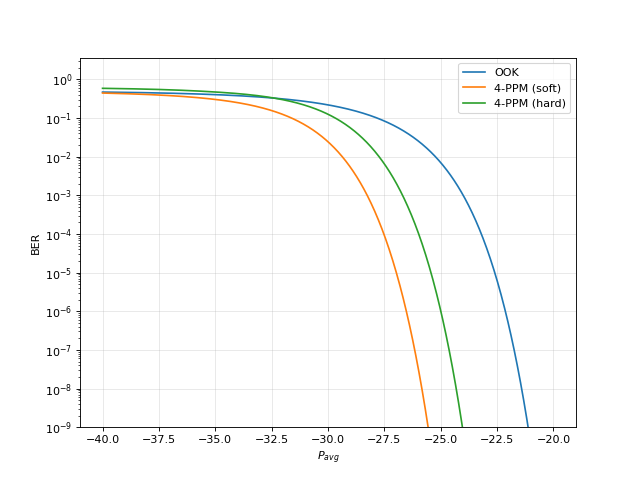
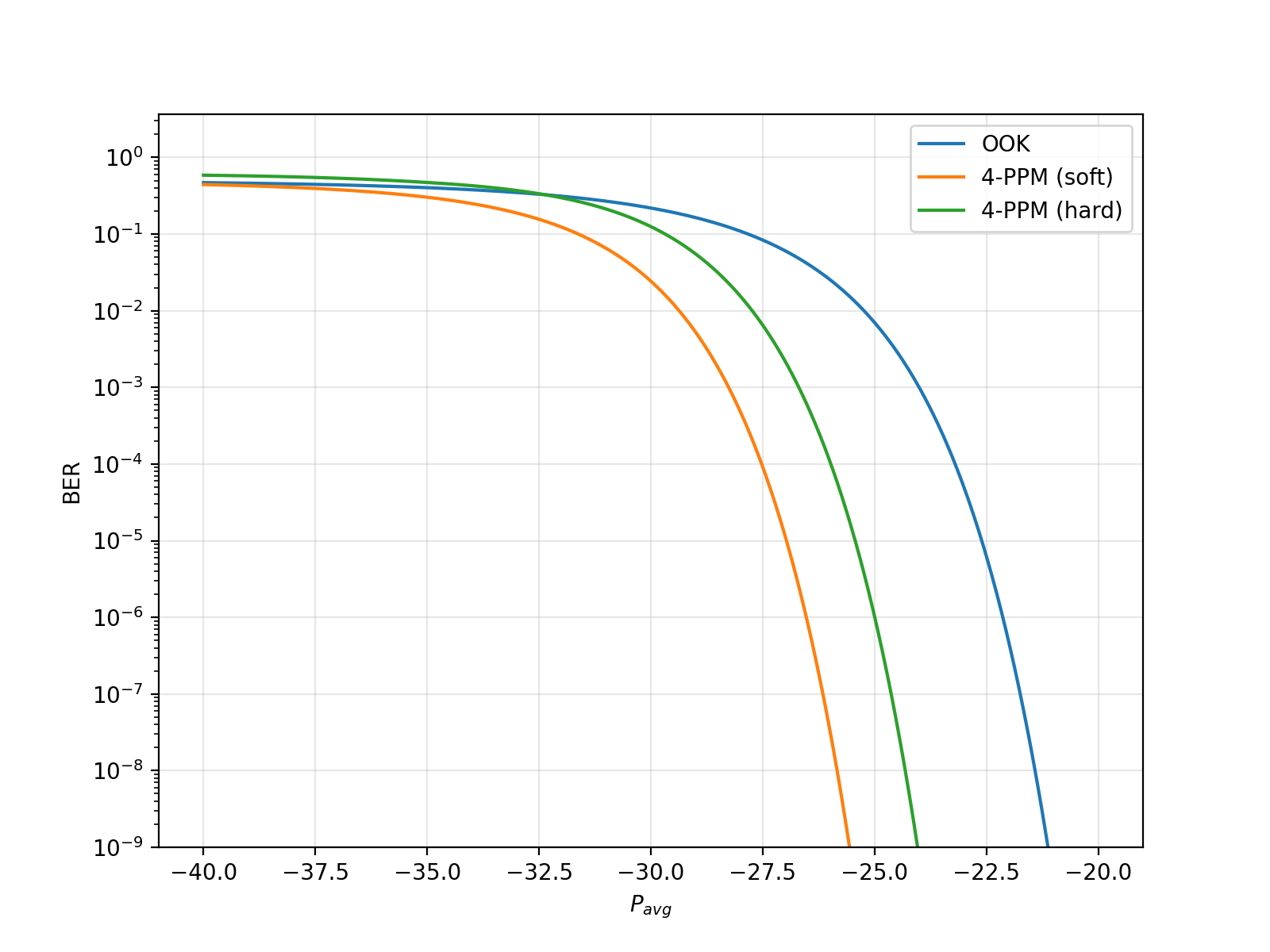
opticomlib.utils.theory_BER(P_avg, modulation: Literal['ook', 'ppm'], M=None, decision=None, threshold=None, ER=inf, amplify=False, f0=193414500000000.0, G=None, NF=None, BW_opt=None, r=1.0, BW_el=5000000000.0, R_L=50, T=300, NF_el=0)

This function calculates the bit error rate (BER) for an OPTICAL RECEIVER, based on a PIN photodetector, from the average input power. It also allows consider the effects of an EDFA amplifier in the results.

If amplify==False, thermal and shot noise of PIN will be consider in BER calculation. If amplify==True, signal-ase and ase-ase beating noises generated by the EDFA are consider too.

In addition, parameter NF_el != 0 (electrical noise figure) can be used to represent another sources of noise after detection, like electrical amplifiers, etc.

Parameters:

• P_avg (float) – Average Received input optical Power (in [dBm]).

• modulation (Literal['ook', 'ppm']) – Kind of modulation format {‘ook’, ‘ppm’}, more modulations in future…

• M (int) – Order of M-ary PPM (a power of 2). Only needed if modulation=’ppm’.

• decision (Literal['hard', 'soft']) – Kind of PPM decision. ‘hard’ decision use the optimum threshold to separate ON and OFF slots. ‘soft’ decision use the Maximum a Posteriori (MAP) and it outperform ‘hard’ decision. Only needed if modulation=’ppm’.

• threshold (float) – Threshold for decision. Only needed if (modulation=’ook’) or (modulation=’ppm and decision=’hard’). Value must be in (0, 1), without include edges. By default optimum threshold is used.

• ER (float) – Extinction Ratio of the input optical signal, in [dB].

• amplify (bool) – If use an EDFA or not at the receiver (before PIN). Default: False.

• f0 (float) – Central frequency of communication, in [Hz]. Only used if amplify=True. Default: 193.4 THz corresponding to 1550 nm.

• G (float) – Gain of EDFA, in [dB]. Only used if amplify=True. This parameter is mandatory.

• NF (float) – Noise Figure of EDFA, in [dB]. Only used if amplify=True. Mandatory.

• BW_opt (float) – Bandwidth of optical filter that is placed after the EDFA, in [Hz]. Only used if amplify=True. Mandatory.

• r (float) – Responsivity of photo-detector. Default: 1.0 [A/W]

• BW_el (float) – Bandwidth of photo-detector or electrical filter, in [Hz]. Default: 5e9 [Hz].

• R_L (float) – Load resistance of photo-detector, in [Ω]. Default: 50 [Ω].

• T (float) – Temperature of photo-detector, in [K]. Default: 300 [K].

• NF_el (float) – Equivalent Noise Figure of electric circuit, in [dB]. Default: 0 [dB]

Returns:

BER – Theoretical Bit Error rate of the system specified.

Return type:

float

Notes

The bandwidths are used only for the determination of the noise contribution to the BER value, i.e. the signal distortion due to these bandwidth is not taken into account. Therefore, the bandwidths BW_el and BW_opt are not considered to affect the transmitted signal.

Example

from opticomlib import theory_BER
import matplotlib.pyplot as plt
import numpy as np

x = np.linspace(-40, -20, 1000)  # Average input optical power [dB]

plt.figure(figsize=(8, 6))

plt.semilogy(x, theory_BER(P_avg=x, modulation='ook'), label='OOK')
plt.semilogy(x, theory_BER(P_avg=x, modulation='ppm', M=4, decision='soft'), label='4-PPM (soft)')
plt.semilogy(x, theory_BER(P_avg=x, modulation='ppm', M=4, decision='hard'), label='4-PPM (hard)')

plt.xlabel(r'$P_{avg}$')
plt.ylabel('BER')
plt.legend()
plt.grid(alpha=0.3)
plt.ylim(1e-9,)
plt.show()

(Source code, png, hires.png, pdf)

opticomlib.utils.shortest_int(x: ndarray, percent: float = 50) → tuple[float, float]

Estimation of the shortest interval of x values, containing {percent}% of the samples in ‘x’.

Parameters:

• x (ndarray) – Data of not complex values. If data is complex, real part will be taken.

• percent (real number) – percent of of data.

Returns:

The shortest interval containing 50% of the samples in ‘data’.

Return type:

tuple[float, float]

opticomlib.utils.apply_optimized_gaussian_filter(t, signal, T_bit)

Applies a Gaussian filter to a NRZ signal. The filter is optimized based on the bit duration, to a sigma of 0.139 * T_bit.

Args:

t (np.ndarray): Time vector corresponding to signal_in. signal (np.ndarray): NRZ input signal. T_bit (float): Bit duration, used as a reference for sigma.

Returns:

np.ndarray: The filtered signal with scaled amplitude.

opticomlib.utils.eyediagram(y, sps, n_traces=None, cmap='viridis', N_grid_bins=350, grid_sigma=3, ax=None, **plot_kw)

Plots a colored eye diagram, internally calculating color density.

Parameters:

• y (np.ndarray) – Full amplitude array (1D).

• sps (int) – Samples per symbol. Used to segment the eye traces.

• n_traces (int, optional) – Maximum number of traces to plot. If None, all available traces will be plotted. Defaults to None.

• cmap (str, optional) – Name of the matplotlib colormap. Defaults to ‘viridis’.

• N_grid_bins (int, optional) – Number of bins for the density histogram. Defaults to 350.

• grid_sigma (float, optional) – Sigma for the Gaussian filter applied to the density. Defaults to 3.

• ax (matplotlib.axes.Axes, optional) – Axes object to plot on. If None, creates new figure and axes. Defaults to None.

• **plot_kw (dict, optional) –

  Additional plotting parameters:

  Figure parameters (used only if ax is None): - figsize : tuple, default (10, 6) - dpi : int, default 100

  Line collection parameters: - linewidth : float, default 0.75 - alpha : float, default 0.25 - capstyle : str, default ‘round’ - joinstyle : str, default ‘round’

  Axes formatting parameters: - xlabel : str, default “Time (2-symbol segment)” - ylabel : str, default “Amplitude” - title : str, default “Eye Diagram ({num_traces} traces)” - grid : bool, default True - grid_alpha : float, default 0.3 - xlim : tuple, optional (xmin, xmax) - ylim : tuple, optional (ymin, ymax) - tight_layout : bool, default True

  Display parameters: - show : bool, default False (whether to call plt.show())

Returns:

The axes object containing the eye diagram plot.

Return type:

matplotlib.axes.Axes

opticomlib.utils.rcos_pulse(beta, span, sps, shape='sqrt')

Generate a raised cosine or root raised cosine filter impulse response.

This function replicates the MATLAB rcosdesign() function, generating the impulse response of a raised cosine or root raised cosine filter used in digital communications for pulse shaping.

Parameters:

• beta (float) – Roll-off factor, must be between 0 and 1.

• span (int) – Number of symbols. The filter length will be span * sps + 1.

• sps (int) – Samples per symbol.

• shape (str, optional) – Filter shape, either ‘normal’ for raised cosine or ‘sqrt’ for root raised cosine. Default is ‘sqrt’.

Returns:

The filter impulse response, normalized to unit energy.

Return type:

numpy.ndarray

Raises:

ValueError – If beta is not in [0, 1] or shape is not ‘normal’ or ‘sqrt’.

Notes

The filter is normalized such that the sum of squares of the coefficients is 1. For beta=0, it reduces to a sinc() function.

Examples

>>> import numpy as np
>>> h = rcos(0.5, 6, 64, 'sqrt')
>>> h.shape
(384,)

opticomlib.utils.gauss_pulse(span, sps, T=1, m=1, c=0.0)

Generate a Gaussian or Super-Gaussian filter.

This function generates the impulse response of a Gaussian filter used in digital communications to reduce bandwidth and minimize intersymbol interference.

Parameters:

• span (int) – Number of symbols. The filter length will be span * sps + 1.

• sps (int) – Samples per symbol.

• T (float) – Full Width at Half Maximum (FWHM) of the pulse in symbols. Default is 1.

• m (int) – Super-Gaussian order. Default is 1 (standard Gaussian).

• c (float) – Chirp parameter. Default is 0.0 (no chirp).

Returns:

The impulse response of the Gaussian filter, normalized to unit energy.

Return type:

numpy.ndarray

Notes

The filter is normalized such that the sum of squares of the coefficients is 1. The Gaussian shape helps reduce intersymbol interference in modulation systems.

Examples

>>> import numpy as np
>>> h = gauss(6, 8, 1.0)
>>> print(h.shape)
(49,)
>>> print('Energy:', np.sum(h**2))
1.0

opticomlib.utils.nrz_pulse(span, sps, T)

Generate a Non-Return-to-Zero (NRZ) pulse shape.

This function generates the impulse response of a Non-Return-to-Zero (NRZ) pulse shape, commonly used in digital communications for pulse shaping.

Parameters:

• span (int) – Number of symbols. The filter length will be span * sps + 1.

• sps (int) – Samples per symbol.

• T (float) – Duration of the NRZ pulse in symbols.

Returns:

The impulse response of the NRZ pulse shape.

Return type:

numpy.ndarray

opticomlib.utils.upfir(x, h, up=1)

Replicate MATLAB’s upfirdn function for upsampling and FIR filtering.

This function performs upsampling of the input signal and then applies an FIR filter, partially replicating the functionality of MATLAB’s upfirdn.

Parameters:

• x (array_like) – Input signal to process.

• h (array_like) – Impulse response of the FIR filter.

• up (int, optional) – Upsampling factor. Default is 1 (no upsampling).

Returns:

The filtered signal after upsampling, convolution and downsampling.

Return type:

numpy.ndarray

Notes

Upsampling is performed by inserting zeros between the input signal samples. Convolution is then applied with the filter using mode=’same’ to maintain length. Finally, downsampling is performed by selecting every dn-th sample from the filtered signal.

opticomlib.utils.phase_estimator(t, x, f)

Estimates the phase and amplitude of a sinusoid with known frequency.

Parameters:

• t (array_like) – Times in seconds, shape (N,).

• x (array_like) – Sampled signal, shape (N,).

• f (float) – Frequency in Hz.

Returns:

• phi (float) – Estimated phase in radians.

• amp (float) – Estimated amplitude.

Notes

The model is \(x[n] = A \cos(2\pi f t[n] + \phi) + noise\), solved by linear regression over \([\cos(\omega t), \sin(\omega t)]\).

opticomlib.utils.get_psd(signal, fs, nperseg=None)

Calculate the Power Spectral Density (PSD) of a signal using Welch’s method.

Parameters:

• signal (Array_Like) – Input signal.

• fs (float) – Sampling frequency in Hz.

• nperseg (int, optional) – Length of each segment for Welch’s method. If None, defaults to 2048 or the length of the signal, whichever is smaller.

Returns:

• f (np.ndarray) – Frequency array.

• psd (np.ndarray) – Power Spectral Density.