Electro-Optical Devices

Use this module to simulate electro-optical devices.

>>> import opticomlib.devices as dv

Devices

PRBS(order[, len, seed, return_seed])	Pseudorandom binary sequence generator
DAC(input[, bias, Vout, pulse_shape, BW])	Digital-to-Analog Converter
PM(op_input, el_input[, Vpi])	Optical Phase Modulator
MZM(op_input, el_input[, bias, Vpi, ...])	Mach-Zehnder modulator
BPF(input, BW[, n])	Optical Band-Pass Filter
EDFA(input, G, NF, BW)	Erbium Doped Fiber
DM(input, D[, retH])	Dispersive Medium
FIBER(input, length[, alpha, beta_2, ...])	Optical Fiber
LPF(input, BW[, n, fs, retH])	Low Pass Filter
PD(input, BW[, r, T, R_load, include_noise, ...])	P-I-N Photodetector
ADC(input[, fs, BW, nbits])	Analog-to-Digital Converter
GET_EYE(input[, nslots, sps_resamp])	Get Eye Parameters Estimator
SAMPLER(input, _eye_)	Digital sampler
FBG(input[, neff, v, landa_D, fc, kL, L, N, ...])	Fiber Bragg Grating.

opticomlib.devices.PRBS(order: Literal[7, 9, 11, 15, 20, 23, 31], len: int = None, seed: int = None, return_seed: bool = False)

Pseudorandom binary sequence generator

Parameters:

• order (int, {7, 9, 11, 15, 20, 23, 31}) – degree of the generating pseudorandom polynomial

• len (int, optional) – lenght of output binary sequence

• seed (int, optional) – seed of the generator (initial state of the LFSR). It must be provided if you want to continue the sequence. Default is 2**order-1.

• return_seed (bool, optional) – If True, the last state of LFSR is returned. Default is False.

Returns:

out – generated pseudorandom binary sequence

Return type:

binary_sequence

Raises:

• ValueError – If order is not in [7, 9, 11, 15, 20, 23, 31].

• TypeError – If len is not an integer.

Warns:

UserWarning – If the seed is 0 or a multiple of 2**order.

Examples

You can generate a PRBS sequence using the following code:

>>> from opticomlib.devices import PRBS
>>> PRBS(order=7, len=10)
binary_sequence([1 0 0 0 0 0 0 1 0 0])
>>> PRBS(order=31, len=20)
binary_sequence([1 0 0 0 0 0 0 0 0 0 0 0 0 0 0 0 0 0 0 0])

You can fix the LFSR iniitial state of generator by using the following code:

>>> PRBS(order=7, len=10, seed=124)
binary_sequence([0 0 0 0 0 1 0 0 0 0])

Notes

For more details, see [prbs].

• \(2^7-1\) bits. Polynomial \(= X^7 + X^6 + 1\)

• \(2^9-1\) bits. Polynomial \(= X^9 + X^5 + 1\)

• \(2^{11}-1\) bits. Polynomial \(= X^{11} + X^9 + 1\)

• \(2^{15}-1\) bits. Polynomial \(= X^{15} + X^{14} + 1\)

• \(2^{20}-1\) bits. Polynomial \(= X^{20} + X^3 + 1\)

• \(2^{23}-1\) bits. Polynomial \(= X^{23} + X^{18} + 1\)

• \(2^{31}-1\) bits. Polynomial \(= X^{31} + X^{28} + 1\)

References

[prbs]

“Pseudorandom binary sequence” https://en.wikipedia.org/wiki/Pseudorandom_binary_sequence

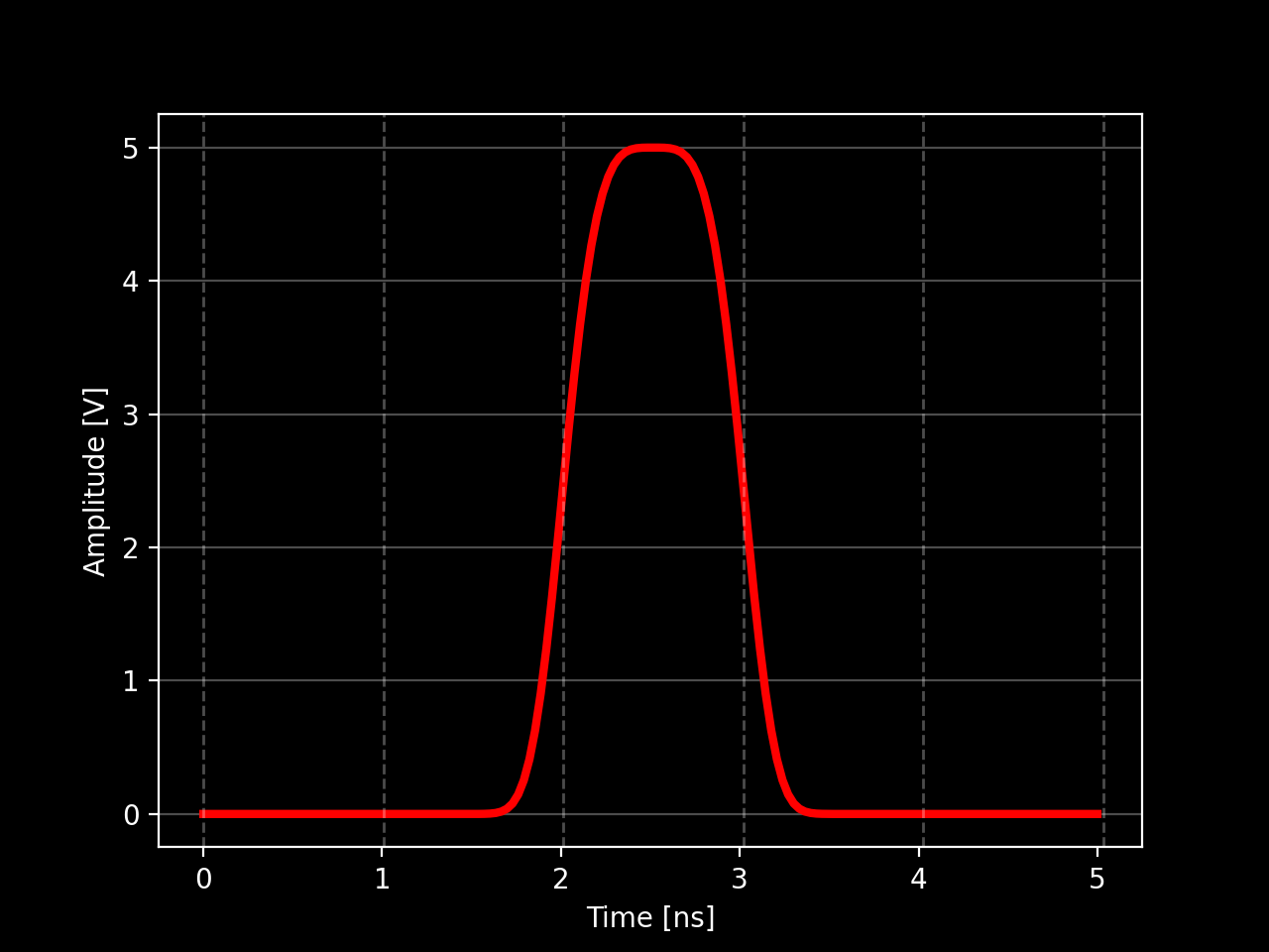
opticomlib.devices.DAC(input: str | list | tuple | ndarray | binary_sequence, bias: float = 0.0, Vout: float = 1.0, pulse_shape: Literal['nrz', 'rz', 'rect', 'gaussian'] = 'nrz', BW: float = None, **kwargs)

Digital-to-Analog Converter

Converts a binary sequence into an electrical signal, sampled at a frequency gv.fs.

Warning

Parameter value pulse_shape='rect' is equivalent to pulse_shape='nrz'. It is recommended to use pulse_shape='nrz', 'rect' will be removed in futures versions.

Parameters:

• input (str, list, tuple, np.ndarray, or binary_sequence) – Input binary sequence.

• bias (float) – DC bias of the output signal. Default: 0.0

• Vout (float) – Output signal amplitude. Should be in the range [-48, 48] Volts. Default: 1.0

• pulse_shape (str, {‘nrz’, ‘rect’, ‘gaussian’}) – Pulse shape at the output. Default: ‘nrz’

• BW (float) – Bandwidth of DAC. If None bandwidth is not limited. Default: None

• c (float) – Chirp of the Gaussian pulse. Only applicable if pulse_shape='gaussian'. Default: 0.0

• m (int) – Order of the super-Gaussian pulse. Only applicable if pulse_shape='gaussian'. Default: 1

• T (int) – Pulse width at half maximum in number of samples. Only applicable if pulse_shape='gaussian'. Default: gv.sps

Returns:

The converted electrical signal.

Return type:

electrical_signal

Raises:

• ValueError – If pulse_shape is not 'rect' or 'gaussian'. If Vout is not between -48 and 48 Volts. If bias is not between -48 and 48 Volts. If T is <=0 or greater than 2 times the samples per bit. If m is not a positive integer.

• TypeError – If Vout is not a scalar value. If bias is not a scalar value. If c is not a scalar value. If m is not an integer value. If T is not an integer value.

Examples

from opticomlib.devices import DAC
from opticomlib import gv

gv(sps=32) # set samples per bit

DAC('0 0 1 0 0', Vout=5, pulse_shape='gaussian', m=2).plot('r', lw=3, grid=True).show()

(Source code, png, hires.png, pdf)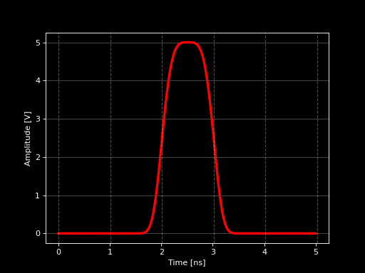

opticomlib.devices.PM(op_input: optical_signal, el_input: float | ndarray | electrical_signal, Vpi: float = 5.0)

Optical Phase Modulator

Modulate the phase of the input optical signal through input electrical signal.

Parameters:

• op_input (optical_signal) – Optical signal to be modulated.

• el_input (float, ndarray, or electrical_signal) – Driver voltage. It can be an integer value, in which case the phase modulation is constant, or an electrical signal of the same length as the optical signal.

• Vpi (float) – Voltage at which the device achieves a phase shift of \(\pi\). Default value is 5.0.

Returns:

op_output – Modulated optical signal.

Return type:

optical_signal

Raises:

• TypeError – If op_input type is not [optical_signal]. If el_input type is not in [float, ndarray, electrical_signal].

• ValueError – If el_input is [ndarray] or [electrical_signal] but, length is not equal to op_input length.

Notes

The output signal is given by:

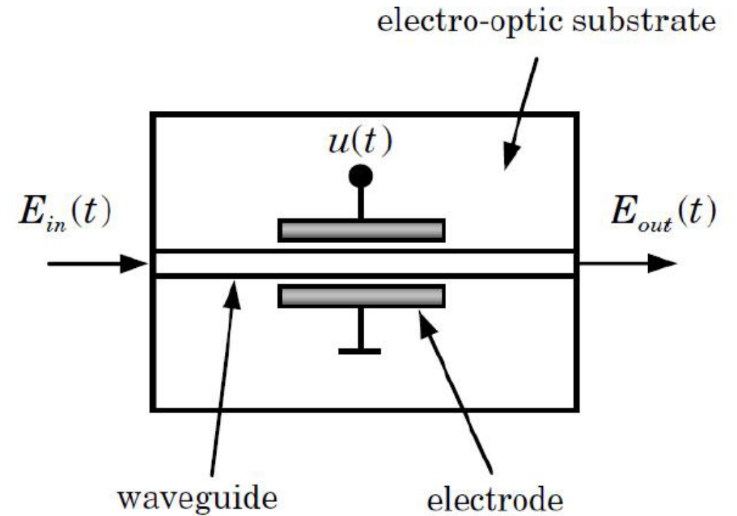\[E_{out} = E_{in} \cdot e^{\left(j\pi \frac{u(t)}{V_{\pi}}\right)}\]

Examples

from opticomlib.devices import PM
from opticomlib import optical_signal, gv
import matplotlib.pyplot as plt
import numpy as np

gv(sps=16, R=1e9) # set samples per bit and bitrate

op_input = optical_signal(np.exp(1j*np.linspace(0,4*np.pi, 1000))) # input optical signal ( exp(j*w*t) )
t = op_input.t()*1e9

fig, axs = plt.subplots(3,1, sharex=True, tight_layout=True)

# Constant phase
output = PM(op_input, el_input=2.5, Vpi=5)

axs[0].set_title(r'Constant phase change ($\Delta f=0$)')
axs[0].plot(t, op_input.signal[0].real, 'r-', label='input', lw=3)
axs[0].plot(t, output.signal[0].real, 'b-', label='output', lw=3)
axs[0].grid()

# Lineal phase
output = PM(op_input, el_input=np.linspace(0,5*np.pi,op_input.len()), Vpi=5)

axs[1].set_title(r'Linear phase change  ($\Delta f \rightarrow cte.$)')
axs[1].plot(t, op_input.signal[0].real, 'r-', label='input', lw=3)
axs[1].plot(t, output.signal[0].real, 'b-', label='output', lw=3)
axs[1].grid()

# Quadratic phase
output = PM(op_input, el_input=np.linspace(0,(5*np.pi)**0.5,op_input.len())**2, Vpi=5)

plt.title(r'Quadratic phase change ($\Delta f \rightarrow linear$)')
axs[2].plot(t, op_input.signal[0].real, 'r-', label='input', lw=3)
axs[2].plot(t, output.signal[0].real, 'b-', label='output', lw=3)
axs[2].grid()

plt.xlabel('Tiempo [ns]')
plt.legend(bbox_to_anchor=(1, 1), loc='upper left')
plt.show()

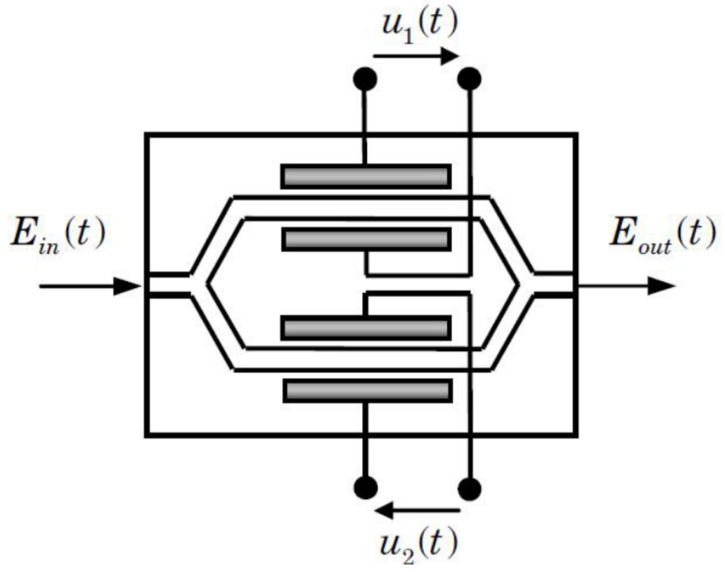
opticomlib.devices.MZM(op_input: optical_signal, el_input: float | ndarray | electrical_signal, bias: float = 0.0, Vpi: float = 5.0, loss_dB: float = 0.0, ER_dB: float = 26.0, pol: Literal['x', 'y'] = 'x', BW: float = None)

Mach-Zehnder modulator

Asymmetric coupler and opposite driving voltages model (\(u_1(t)=-u_2(t)=u(t)\) Push-Pull configuration). The input and output are polarization maintained. Internally, the modulator can select the polarization to be modulated by setting the parameter pol to 'x' or 'y'. If one of them is selected, the other is strongly attenuated (set to zeros).

Parameters:

• op_input (optical_signal) – Optical signal to be modulated. This optical signal must contain only one polarization op_input.n_pol=1. Otherwise it remove the second polarization.

• el_input (Number, ndarray, or electrical_signal) – Driver voltage, with zero bias.

• bias (float, optional) – Modulator bias voltage. Default is 0.0.

• Vpi (float, optional) – Voltage at which the device switches from on-state to off-state. Default is 5.0 V.

• loss_dB (float, optional) – Propagation or insertion losses in the modulator, value in dB. Default is 0.0 dB.

• ER_dB (float, optional) – Extinction ratio of the modulator, in dB. Default is 26 dB.

• pol (str, {‘x’, ‘y’} optional) – Polarization of the modulator. Default is 'x'.

• BW (float, optional) – Modulator bandwidth in Hz. If not provided, the bandwidth is not limited.

Returns:

Modulated optical signal.

Return type:

optical_signal

Raises:

• TypeError – If op_input type is not [optical_signal]. If el_input type is not in [float, ndarray, electrical_signal].

• ValueError – If el_input is [ndarray] or [electrical_signal] but, length is not equal to op_input length.

Notes

The output signal is given by [1]:

\[\vec{E}_{out} = \vec{E}_{in} \cdot \sqrt{l} \cdot \left[ \cos\left(\frac{\pi}{2V_{\pi}}(u(t)+V_{bias})\right) + j \frac{\eta}{2} \sin\left(\frac{\pi}{2V_{\pi}}(u(t)+V_{bias})\right) \right]\]

where \(\eta = 2\times 10^{-ER_{dB}/10}\) and \(l = 10^{-loss_{dB}/10}\).

References

[1]

Tetsuya Kawanishi, “Electro-optic Modulation for Photonic Networks”, Chapter 4.3 (2022). doi: https://doi.org/10.1007/978-3-030-86720-1

Examples

from opticomlib import idbm, dbm, optical_signal, gv
from opticomlib.devices import MZM

import numpy as np
import matplotlib.pyplot as plt

gv(sps=128, R=10e9) # set samples per bit and bitrate

Vpi = 5
tx_seq = np.array([0, 1, 0, 1, 0, 0, 1, 1, 0, 0], bool)

V = DAC(~tx_seq, Vout=Vpi, pulse_shape='rect') - Vpi/2

input = optical_signal( np.ones_like(V.signal)*idbm(10)**0.5 )
input.noise = np.random.normal(0, 0.01, input.len())
t = input.t()*1e9

mod_sig = MZM(input, el_input=V, bias=Vpi/2, Vpi=Vpi, loss_dB=2, ER_dB=40, BW=40e9)

fig, axs = plt.subplots(3,1, sharex=True, tight_layout=True)

# Plot input and output power
axs[0].plot(t, dbm(input.abs()**2), 'r-', label='input', lw=3)
axs[0].plot(t, dbm(mod_sig.abs()**2), 'C1-', label='output', lw=3)
axs[0].legend(bbox_to_anchor=(1, 1), loc='upper left')
axs[0].set_ylabel('Potencia [dBm]')
for i in t[::gv.sps]:
    axs[0].axvline(i, color='k', linestyle='--', alpha=0.5)

# # Plot fase
phi_in = input.phase()
phi_out = mod_sig.phase()

axs[1].plot(t, phi_in, 'b-', label='Fase in', lw=3)
axs[1].plot(t, phi_out, 'C0-', label='Fase out', lw=3)
axs[1].set_ylabel('Fase [rad]')
axs[1].legend(bbox_to_anchor=(1, 1), loc='upper left')
for i in t[::gv.sps]:
    axs[1].axvline(i, color='k', linestyle='--', alpha=0.5)

# Frecuency chirp
freq_in = 1/2/np.pi*np.diff(phi_in)/np.diff(t)
freq_out = 1/2/np.pi*np.diff(phi_out)/np.diff(t)

axs[2].plot(t[:-1], freq_in, 'k', label='Frequency in', lw=3)
axs[2].plot(t[:-1], freq_out, 'C7', label='Frequency out', lw=3)
axs[2].set_xlabel('Tiempo [ns]')
axs[2].set_ylabel('Frequency Chirp [Hz]')
axs[2].legend(bbox_to_anchor=(1, 1), loc='upper left')
for i in t[::gv.sps]:
    axs[2].axvline(i, color='k', linestyle='--', alpha=0.5)
plt.show()

opticomlib.devices.BPF(input: optical_signal, BW: float, n: int = 4)

Optical Band-Pass Filter

Filters the input optical signal, allowing only the desired frequency band to pass. Bessel filter model.

Parameters:

• input (optical_signal) – The optical signal to be filtered.

• BW (float) – The bandwidth of the filter in Hz.

• n (int, default: 4) – The order of the filter.

Returns:

The filtered optical signal.

Return type:

optical_signal

opticomlib.devices.EDFA(input: optical_signal, G: float, NF: float, BW: float)

Erbium Doped Fiber

Amplifies the optical signal at the input, adding amplified spontaneous emission (ASE) noise. Simplest model (no saturation output power).

Parameters:

• input (optical_signal) – The optical signal to be amplified.

• G (float) – The gain of the amplifier, in dB.

• NF (float) – The noise figure of the amplifier, in dB.

• BW (float) – The bandwidth of the amplifier, in Hz.

Returns:

The amplified optical signal.

Return type:

optical_signal

Raises:

TypeError – If input is not an optical_signal.

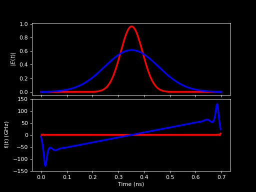
opticomlib.devices.DM(input: optical_signal, D: float, retH: bool = False)

Dispersive Medium

Emulates a medium with only the dispersion property, i.e., only \(\beta_2\) different from zero.

Parameters:

• input (optical_signal) – The input optical signal.

• D (float) – The dispersion coefficient of the medium (\(\beta_2z\)), in [ps^2].

• retH (bool, default: False) – If True, the frequency response of the medium is also returned.

Returns:

• optical_signal – The output optical signal.

• H (ndarray) – The frequency response of the medium. If retH=True.

Raises:

TypeError – If input is not an optical signal.

Notes

Frequency response of the medium is given by:

\[H(\omega) = e^{-j \frac{D}{2} \omega^2}\]

The output signal is simply a fase modulation in the frequency domain of the input signal:

\[E_{out}(t) = \mathcal{F}^{-1} \left\{ H(\omega) \cdot \mathcal{F} \left\{ E_{in}(t) \right\} \right\}\]

Example

from opticomlib.devices import DM, DAC
from opticomlib import optical_signal, gv, idbm, bode

import matplotlib.pyplot as plt
import numpy as np

gv(N=7, sps=32, R=10e9)

signal = DAC('0,0,0,1,0,0,0', pulse_shape='gaussian')
input = optical_signal( signal.signal/signal.power()**0.5*idbm(20)**0.5, n_pol=2 )

output, H = DM(input, D=4000, retH=True)

t = gv.t*1e9

plt.style.use('dark_background')
fig, ax = plt.subplots(2, 1, sharex=True, gridspec_kw={'hspace': 0.05})

ax[0].plot(t, input.abs()[0], 'r-', lw=3, label='input')
ax[0].plot(t, output.abs()[0], 'b-', lw=3, label='output')

ax[0].set_ylabel(r'$|E(t)|$')

ax[1].plot(t[:-1], np.diff(input.phase()[0])/gv.dt*1e-9, 'r-', lw=3)
ax[1].plot(t[:-1], np.diff(output.phase()[0])/gv.dt*1e-9, 'b-', lw=3)

plt.xlabel('Time (ns)')
plt.ylabel(r'$f_i(t)$ (GHz)')
plt.ylim(-150, 150)
plt.show()

(Source code, png, hires.png, pdf)

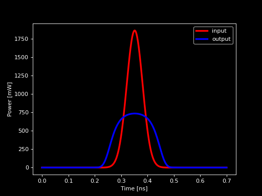
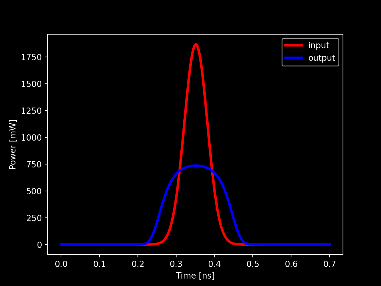
opticomlib.devices.FIBER(input: optical_signal, length: float, alpha: float = 0.0, beta_2: float = 0.0, beta_3: float = 0.0, gamma: float = 0.0, phi_max: float = 0.05, show_progress=False)

Optical Fiber

Simulates the transmission through an optical fiber, solving Schrödinger’s equation numerically, by using split-step Fourier method with adaptive step (method based on limiting the nonlinear phase rotation) [2]. Polarization mode dispersion (PMD) is not considered in this model.

Parameters:

• input (optical_signal) – Input optical signal.

• length (float) – Length of the fiber, in [km].

• alpha (float, default: 0.0) – Attenuation coefficient of the fiber, in [dB/km].

• beta_2 (float, default: 0.0) – Second-order dispersion coefficient of the fiber, in [ps^2/km].

• beta_3 (float, default: 0.0) – Third-order dispersion coefficient of the fiber, in [ps^3/km].

• gamma (float, default: 0.0) – Nonlinearity coefficient of the fiber, in [(W·km)^-1].

• phi_max (float, default: 0.05) – Upper bound of the nonlinear phase rotation, in [rad].

• show_progress (bool, default: False) – Show algorithm progress bar.

Returns:

Output optical signal.

Return type:

optical_signal

Raises:

TypeError – If input is not an optical signal.

References

[2]

O.V. Sinkin; R. Holzlohner; J. Zweck; C.R. Menyuk, “Optimization of the split-step Fourier method in modeling optical-fiber communications systems,” vol. 21, no. 1, pp. 61-68, Jan. 2003, doi: https://doi.org/10.1109/JLT.2003.808628

Example

from opticomlib.devices import FIBER, DAC
from opticomlib import optical_signal, gv, idbm

gv(sps=32, R=10e9)

signal = DAC('0,0,0,1,0,0,0', pulse_shape='gaussian')
input = optical_signal( signal.signal/signal.power()**0.5*idbm(20)**0.5, n_pol=2)

output = FIBER(input, length=50, alpha=0.01, beta_2=-20, gamma=0.1, show_progress=True)

input.plot('r-', label='input', lw=3)
output.plot('b-', label='output', lw=3).show()

(Source code, png, hires.png, pdf)

The input signal is a 10 Gbps NRZ signal with 20 dBm of power. The fiber has a length of 50 km, an attenuation of 0.01 dB/km, a second-order dispersion of -20 ps^2/km, and a nonlinearity coefficient of 0.1 (W·km)^-1. The output signal is shown in blue.

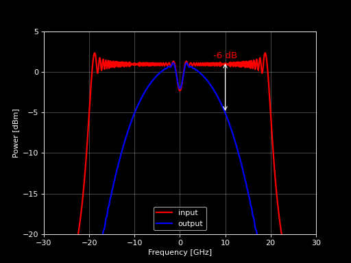
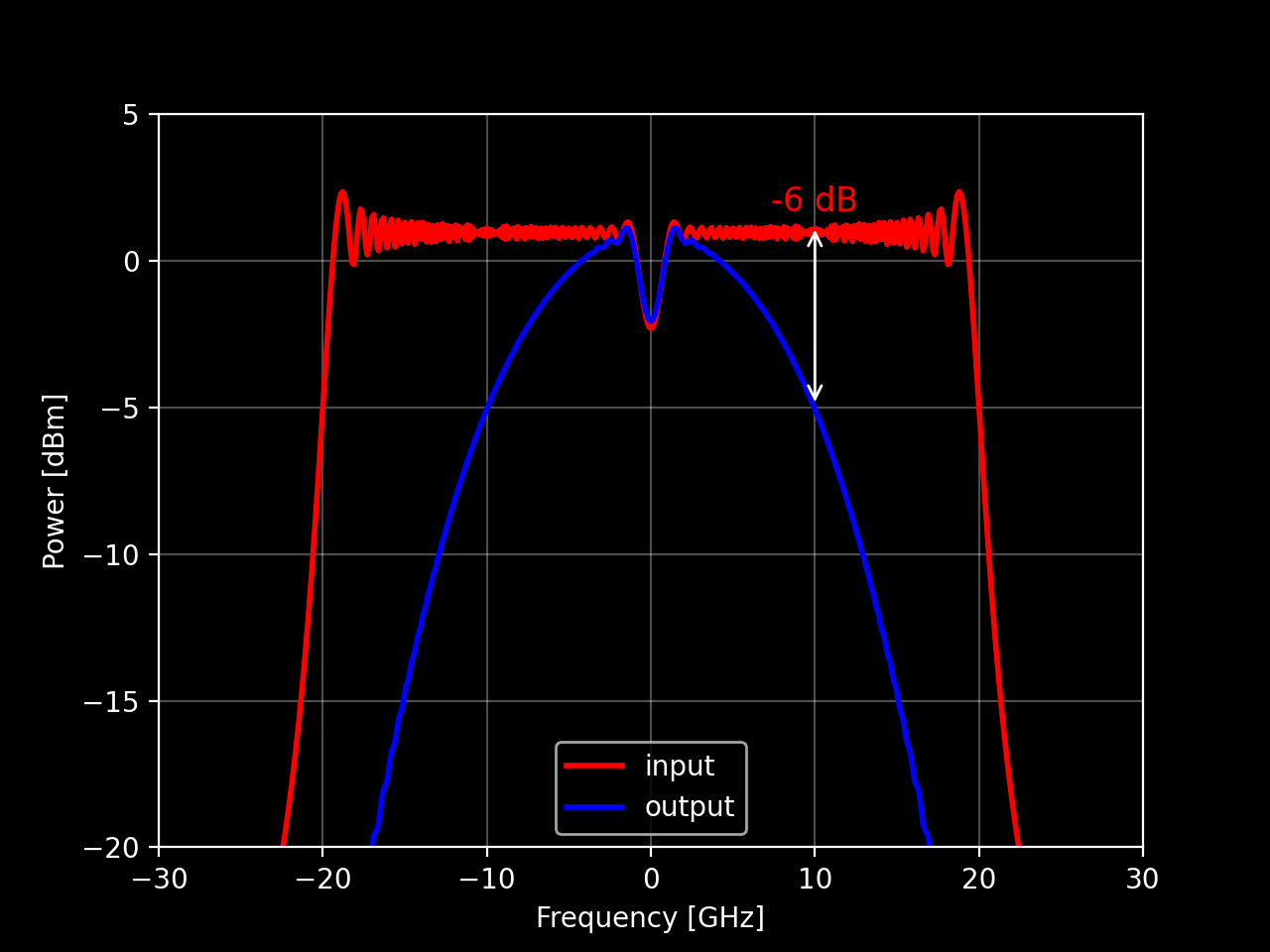
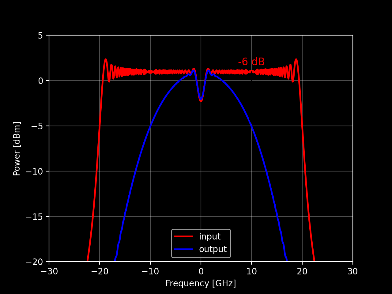
opticomlib.devices.LPF(input: ndarray | electrical_signal, BW: float, n: int = 4, fs: float = None, retH: bool = False)

Low Pass Filter

Filters the input electrical signal, allowing only the desired frequency band to pass. Bessel filter model.

Parameters:

• input (ndarray or electrical_signal) – Electrical signal to be filtered.

• BW (float) – Filter bandwidth or cutoff frequency, in [Hz].

• n (int, default: 4) – Filter order.

• fs (float, default: gv.fs) – Sampling frequency of the input signal.

• retH (bool, default: False) – If True, the frequency response of the filter is also returned.

Returns:

Filtered electrical signal.

Return type:

electrical_signal

Raises:

TypeError – If input is not of type ndarray or electrical_signal.

Example

from opticomlib.devices import LPF
from opticomlib import gv, electrical_signal
import matplotlib.pyplot as plt
import numpy as np

gv(N = 10, sps=128, R=1e9)

t = gv.t
c = 20e9/t[-1]   # frequency chirp from 0 to 20 GHz

input = electrical_signal( np.sin( np.pi*c*t**2) )
output = LPF(input, 10e9)

input.psd('r', label='input', lw=2)
output.psd('b', label='output', lw=2)

plt.xlim(-30,30)
plt.ylim(-20, 5)
plt.annotate('-6 dB', xy=(10, -5), xytext=(10, 2), c='r', arrowprops=dict(arrowstyle='<->'), fontsize=12, ha='center', va='center')
plt.show()

(Source code, png, hires.png, pdf)

opticomlib.devices.PD(input: optical_signal, BW: float, r: float = 1.0, T: float = 300.0, R_load: float = 50.0, include_noise: Literal['ase-only', 'thermal-only', 'shot-only', 'ase-thermal', 'ase-shot', 'thermal-shot', 'all'] = 'all', i_dark: float = 1e-08, Fn=0)

P-I-N Photodetector

Simulates the detection of an optical signal by a P-I-N photodetector.

Parameters:

• input (optical_signal) – Optical signal to be photodetected.

• BW (float) – Detector bandwidth in [Hz].

• r (float, optional) – Detector responsivity in [A/W]. Default: 1.0.

• T (float, optional) – Detector temperature in [K]. Default: 300.0.

• R_load (float, optional) – Detector load resistance in [\(\Omega\)]. Default: 50.0.

• include_noise (str, optional) –

  Type of noise to include in the simulation. Default: ‘all’. Options include:

  • 'ase-only': only include ASE noise

  • 'thermal-only': only include thermal noise

  • 'shot-only': only include shot noise

  • 'ase-thermal': include ASE and thermal noise

  • 'ase-shot': include ASE and shot noise

  • 'thermal-shot': include thermal and shot noise

  • 'all': include all types of noise

• i_dark (float, optional) – Dark current of the photodetector in [A]. Default: 10e-9 [10 nA].

• Fn (float, optional) – Noise figure of Photodetector amplifiers states, in [dB]. Default: 0 dB

Returns:

The detected electrical signal.

Return type:

electrical_signal

Raises:

• TypeError – If input is not of type optical_signal. If r, T, or R_load are not scalar values. If include_noise is not a string.

• ValueError – If r is not between (0, 1]. If T or R_load are negative values. If include_noise argument is not one of the valid options.

Notes

The total photodetected current is given by:

\[i_{ph} = \mathcal{R}P_{in} + i_{th} + i_{sh} + i_{dark}\]

where \(\mathcal{R}\) is the responsivity of the photodetector, \(P_{in}\) is the input power, \(i_{th}\) and \(i_{sh}\) are thermal and shot noise respectively and \(i_{dark}\) is the dark current of photodetector.

The input power \(P_{in}\) is determinated as:

\[\begin{split}P_{in} &= |E_x + n_x|^2 + |E_y + n_y|^2 \\ P_{in} &= |E_x|^2 + |E_y|^2 + 2\Re\{E_x n_x^* + E_y n_y^*\} + |n_x|^2 + |n_y|^2 \\ P_{in} &= P_{sig} + P_{sig-noise} + P_{noise} \\\end{split}\]

where \(E_x\) and \(E_y\) are the amplitudes of x-polarization and y-polarization modes respectively and \(n_x\) and \(n_y\) are the noise of x-polarization and y-polarization modes respectively.

The thermal and shot noises are random variables with normal distribution and variance given by [Agrawal]:

\[\begin{split}\sigma_{th}^2 &= \frac{4k_B T}{R_L}F_n \Delta f \\ \sigma_{sh}^2 &= 2e\left( r(P_{sig}^2 + P_{noise}^2) + i_{dark} \right)\Delta f\end{split}\]

where \(k_B\) is the Boltzmann constant, \(T\) is the temperature of the photodetector, \(R_L\) is the load resistance, \(F_n\) is the noise figure of the photodetector, \(\Delta f\) is the bandwidth of the photodetector, \(e\) is the electron charge.

\[\begin{split}i_{ph} &= \mathcal{R}P_{sig} + \mathcal{R}P_{sig-noise} + \mathcal{R}P_{noise} + i_{th} + i_{sh} + i_{dark} \\ i_{ph} &= i_{sig} + i_{sig-noise} + i_{noise-noise} + i_{th} + i_{sh} + i_{dark}\end{split}\]

References

[Agrawal]

Agrawal, G.P., “Fiber-Optic Communication Systems”. Chapter 4.4 (1997).

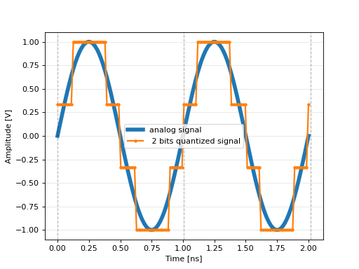
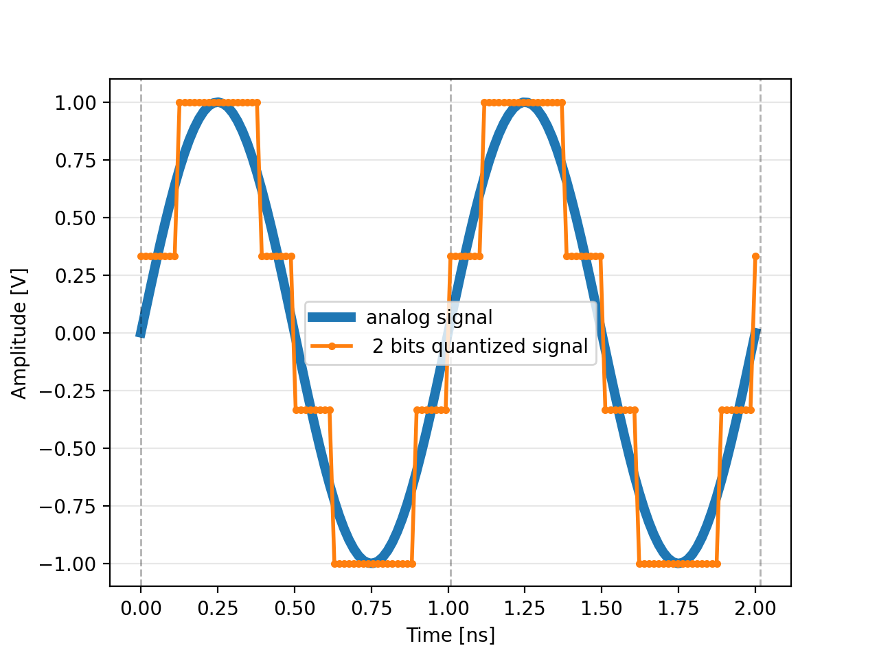
opticomlib.devices.ADC(input: electrical_signal, fs: float = None, BW: float = None, nbits: int = 8) → binary_sequence

Analog-to-Digital Converter

Converts an analog electrical signal into a quantized digital signal, sampled at a frequency fs and filtered with a bandwidth BW.

Parameters:

• input (electrical_signal) – Electrical signal to be quantized.

• fs (float, default: None) – Sampling frequency of the output signal.

• BW (float, default: None) – ADC bandwidth in Hz.

• nbits (int, default: 8) – Vertical resolution of the ADC, in bits.

Returns:

Quantized digital signal.

Return type:

electrical_signal

Raises:

TypeError – If the input is not of type electrical_signal.

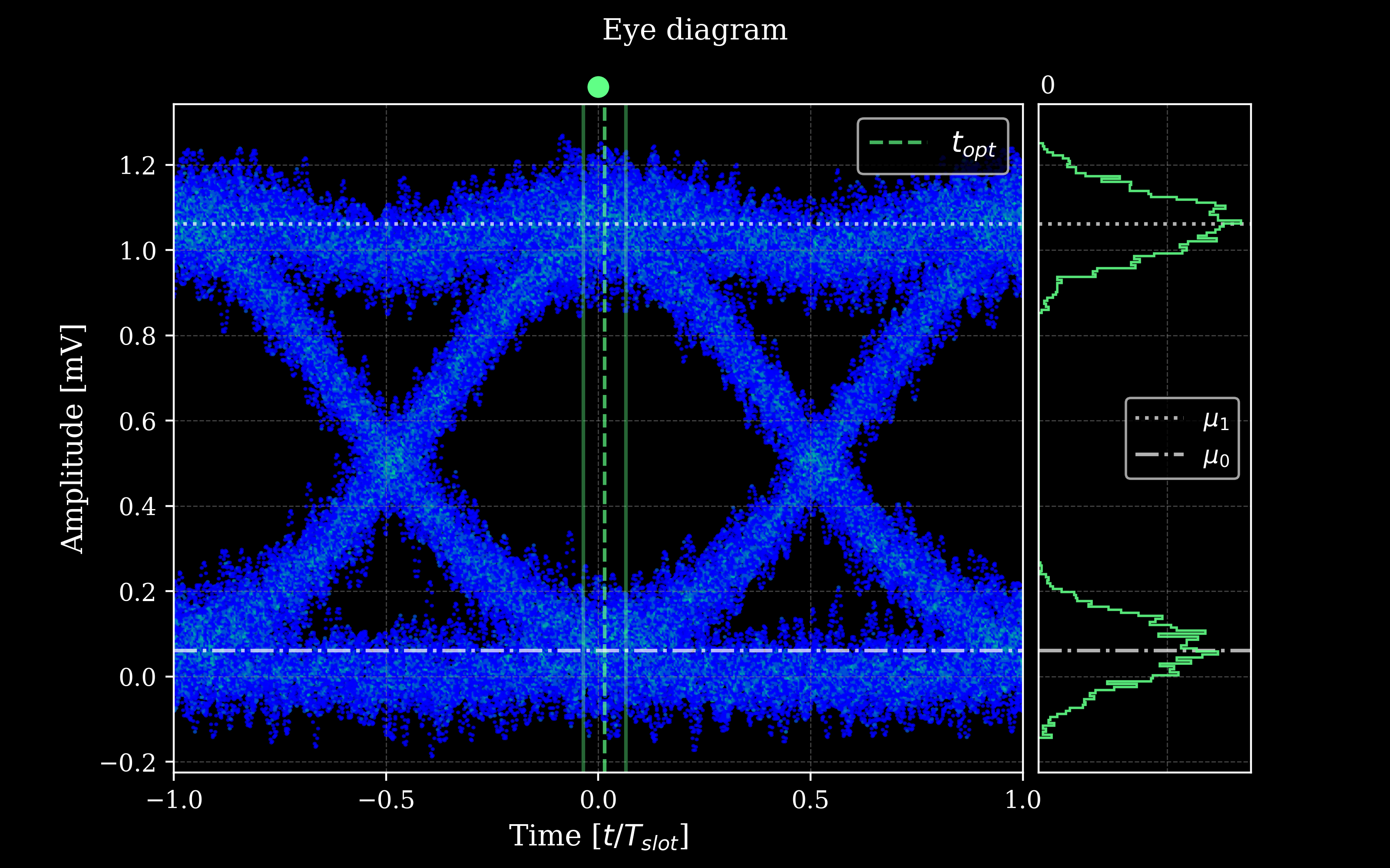
opticomlib.devices.GET_EYE(input: electrical_signal | ndarray, nslots: int = 4096, sps_resamp: int = None)

Get Eye Parameters Estimator

Estimates all the fundamental parameters and metrics of the eye diagram of the input electrical signal.

Parameters:

• input (electrical_signal | np.ndarray) – Electrical or optical signal from which the eye diagram will be estimated.

• nslots (int, default: 4096) – Number of slots to consider for eye reconstruction.

• sps_resamp (int, default: None) – Number of samples per slot to interpolate the original signal.

Returns:

Object of the eye class with all the parameters and metrics of the eye diagram.

Return type:

eye

Raises:

• ValueError – If the input is a ndarray but dimention is >2.

• TypeError – If the input is not of type electrical_signal, optical_signal or np.ndarray.

Example

from opticomlib.devices import PRBS, DAC, GET_EYE
from opticomlib import gv
import numpy as np

gv(sps=64, R=1e9)

y = DAC( PRBS(), pulse_shape='gaussian')
y.noise = np.random.normal(0, 0.05, y.len())

GET_EYE(y, sps_resamp=512).plot() # with interpolation

opticomlib.devices.SAMPLER(input: electrical_signal, _eye_: eye)

Digital sampler

Receives an electrical signal and an eye object and performs the sampling of the signal at the optimal instant determined by the eye object.

Args:

input: The electrical signal to be sampled. _eye_: The eye object that contains the eye diagram information.

Returns:

electrical_signal: The sampled electrical signal at one sample per slot.

opticomlib.devices.FBG(input: optical_signal, neff: float = 1.45, v: float = 1.0, landa_D: float = None, fc: float = None, kL: float = None, L: float = None, N: int = None, dneff: float = None, vdneff: float = None, apodization: Literal['uniform', 'rcos', 'gaussian', 'parabolic'] | Callable = 'uniform', F: float = 0, print_params: bool = True, filtfilt: bool = True, retH: bool = False)

Fiber Bragg Grating.

This function numerically calculates the reflectivity (transfer function \(H(f)\) in reflection) of the grating by solving the coupled-wave equations using Runge-Kutta method with help of signal.integrate.solve_ivp() function. See Notes section for more details.

In order to design the grating, combination of the following parameters can be used:

1. neff, v, fc, (dneff or vdneff), (N or kL or L)

2. neff, v, landaD, (dneff or vdneff), (N or kL or L)

3. neff, v, landaD, kL, (N or L)

Bandwidth is governed essentially by three parameters:

1. Bragg wavelength (\(\lambda_D\)). Bandwidth is proportional to \(\lambda_D\).

2. Product of visibility and effective index change (\(v\delta n_{eff}\)). If \(v\delta n_{eff}\) is small, the bandwidth is small.

3. Length of the grating (\(L\)). Bandwidth is inversely proportional to \(L\).

On the other hand, chirp parameter \(F\) can increase the bandwidth of the grating as well.

Parameters:

• input (optical_signal) – The input optical signal.

• neff (float, optional) – Effective refractive index of core fiber. Default is 1.45.

• v (float, optional) – Visibility of the grating. Default is 1.

• landa_D (float, optional) – Bragg wavelength (resonance wavelength). Default is None.

• fc (float, optional) – Center frequency of the grating. Default is None.

• kL (float, optional) – Product of the coupling coefficient and the length of the grating. Default is None.

• L (float, optional) – Length of the grating. Default is None.

• N (int, optional) – Number of period along grating length. Default is None.

• dneff (float, optional) – Effective index change. Default is None.

• vdneff (float, optional) – Effective index change multiplied by visibility (case of approximation σ->0). Default is None.

• apodization (str or callable) –

  Apodization function. Can be an string with the name of the apodization function or a custom function. Default is 'uniform'.

  The following apodization functions are available:

  • 'uniform': Uniform apodization, f(z) = 1.

  • 'rcos': Raised cosine apodization, f(z) = 1/2*(1 + np.cos(pi*z)).

  • 'gaussian': Gaussian apodization, f(z) = np.exp(-4*np.log(2)*(3*z)**2).

  • 'parabolic': Parabolic apodization, f(z) = 1 - (2*z)**2.

  If a custom function is used, it must be a function of the form f(z) where z is the position along the grating length normalized by L (i.e. z = z/L), and the function must be defined in the range -0.5 <= z <= 0.5.

• F (float, optional) – Chirp parameter. Default is 0.

• filtfilt (bool, optional) – If True, group delay will be corrected in output signal. Default is True.

• retH (bool, optional) – If True, the function will return the reflectivity (H(w)) of the grating. Default is False.

Returns:

• output (optical_signal) – The reflected optical signal

• H (np.ndarray, optional) – Frequency response of grating fiber H(w), only returned if retH=True

Raises:

• TypeError – If input is not an optical_signal.

• ValueError – If the parameters are not correctly specified.

Warns:

• UserWarning – If the apodization function is not recognized, a warning will be issued and the function will use uniform apodization.

• UserWarning – If bandwith is too large, the function will issue a warning and will use a default bandwidth of fs.

Notes

Following coupled-wave theory, we assume a periodic, single-mode waveguide with an electromagnetic field which can be represented by two contradirectional coupled waves in the form [3]:

\[E(z) = A(z)e^{-j\beta_0 z} + B(z)e^{j\beta_0 z}\]

where A and B are slowly varying amplitudes of mode traveling in \(+z\) and math:-z directions, respectively These amplitudes are linked by the standard coupled-wave equations:

\[\begin{split}R' &= j\hat{\sigma} R + j\kappa S \\ S' &= -j\hat{\sigma} S - j\kappa R\end{split}\]

where \(R\) and \(S\) are \(R(z) = A(z)e^{j\delta z - \phi/2}\) and \(S(z) = B(z)e^{-j\delta z + \phi/2}\). In these equations \(\kappa\) is the “AC” coupling coefficient and \(\hat{\sigma}\) is a general “dc” self-coupling coefficient defined as

\[\hat{\sigma} = \delta + \sigma - \frac{1}{2}\phi'\]

The detuning \(\delta\), which is independent of \(z\) for all gratings, is defined to be

\[\delta = 2\pi n_{eff} \left( \frac{1}{\lambda} - \frac{1}{\lambda_{D}} \right)\]

where \(\lambda_D = 2n_{eff}\Lambda\) is the “design wavelength” for Bragg scattering by an infinitesimally weak grating \((\delta n_{eff}\rightarrow 0)\) with a period \(\Lambda\).

For a single-mode Bragg reflection grating:

\[\begin{split}\sigma &= \frac{2\pi}{\lambda}\delta n_{eff} \\ \kappa &= \frac{v}{2}\sigma = \frac{\pi}{\lambda}v\delta n_{eff}\end{split}\]

If the grating is uniform along \(z\), then \(\delta n_{eff}\) is a constant and \(\phi' = 0\), and thus \(\kappa\), \(\sigma\), and \(\hat{\sigma}\) constants.

For apodized gratings, \(\delta n_{eff}\) is a function of \(z\), and therefore \(\kappa\), \(\sigma\), and \(\hat{\sigma}\) are also functions of \(z\).

If phase chirp is present, \(\phi\) and \(\phi'\) are also a function of \(z\). This implementation considers only linear chirp, so:

\[\phi'(z) = 2Fz/L^2\]

where \(F\) is a dimensionless “chirp parameter”, given by [4]:

\[F = \pi N \Delta \Lambda/\Lambda\]

or

\[F = \pi N \Delta \lambda_D/\lambda_D = 2\pi n_{eff} \frac{\Delta \lambda_D}{\lambda_D^2}L\]

where

\[\Delta \lambda_D = \lambda_D(z=-L/2) - \lambda_D(z=L/2)\]

ODE resolution is performed using scipy.integrate.solve_ivp function:

• Dimensionless variables are used: \(z = z/L\), \(\delta = \delta L\), \(\kappa = \kappa L\), \(\sigma = \sigma L\), \(\phi' = \phi' L\).

• The integration is performed from \(z = 1/2\) to \(z = -1/2\).

• The initial conditions are \(R(1/2) = 1\) and \(S(1/2) = 0\).

• The output is the relation \(\rho = S(-1/2)/R(-1/2)\).

References

[3]

Turan Erdogan, “Fiber Grating Spectra,” VOL. 15, NO. 8, AUGUST 1997. doi: https://doi.org/10.1109/50.618322

[4]

8. KOGELNIK, “Filter Response of Nonuniform Almost-Periodic Structures” Vol. 55, No. 1, January 1976. doi: https://doi.org/10.1002/j.1538-7305.1976.tb02062.x

Examples

from opticomlib import optical_signal, gv, pi, db, plt, np
from opticomlib.devices import FBG

gv(fs=100e9)

x = optical_signal(np.ones(2**12))
f = x.w(shift=True)/2/pi*1e-9

for apo in ['uniform', 'parabolic', 'rcos', 'gaussian']:
    _,H = FBG(x, fc=gv.f0, vdneff=1e-4, kL=16, apodization=apo, retH=True)
    plt.plot(f, db(np.abs(H)**2), lw=2, label=apo)

plt.xlabel('Frequency (Hz)')
plt.ylabel('Magnitude (dB)')
plt.legend()
plt.grid(alpha=0.3)
plt.ylim(-100,)
plt.xlim(-20, 20)
plt.show()