Installation
To use Opticomlib, python >=3.10 is required.
Note
If you don’t have python installed, it’s strongly recommended to install it using Miniconda for simplicity in managing packages and environments.
Here is an example for installing Miniconda on Windows (for other OS, please refer to the official documentation),
Open a terminal and run the following commands:
$ curl https://repo.anaconda.com/miniconda/Miniconda3-latest-Windows-x86_64.exe -o miniconda3.exe
$ start /wait "" miniconda3.exe
$ del miniconda3.exe
After installing, open the “Anaconda Prompt (miniconda3)” program to use Miniconda3. Then you can create
a new environment and install Opticomlib using the following commands:
(base)$ conda create -n optic_env python=3.10
(base)$ conda activate optic_env
(optic_env)$ pip install opticomlib
If you want to install an specific branch of the git repository, you can use the following command:
(optic_env)$ pip install git+https://github.com/armando-palacio/opticomlib.git@branch_name
Usage
To use library, you have to import the modules you need (as devices, ook, ppm, etc) and use them in your code.
Also, you need to import gv variable from any module or opticomlib directly, in order to set global variables for simulation.
Here there are some examples of how to use Opticomlib.
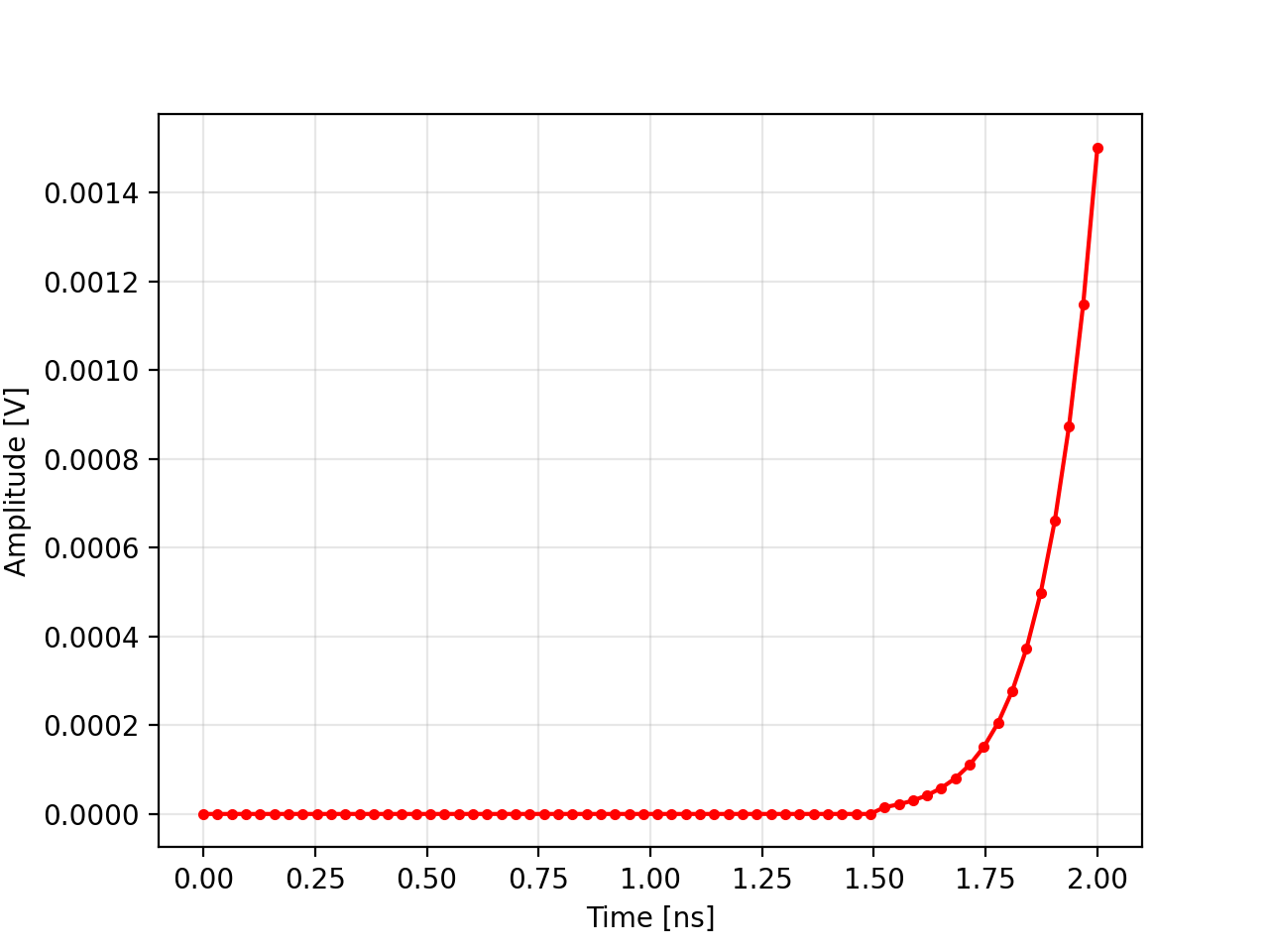
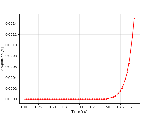
Generate a gaussian pulse with a given width and amplitude is so easy using
DAC()device.
from opticomlib.devices import DAC, gv

gv(sps=32, R=1e9) # set samples per slot and slot rate, it automatically will set de sampling frequency (fs),
                  # see "Data Types/global_variables" documentation page for more details

pulse = DAC('0001000', pulse_shape='gaussian', Vpp=1) # create a gaussian pulse with 1V of amplitude peak-to-peak
                                                      # see "Devices/DAC" documentation page for more details

pulse.plot('r.-').grid().show() # plot, grid and show the pulse,
                                # see "Data Types/electrical_signal.plot" documentation page for more details
(Source code, png, hires.png, pdf)
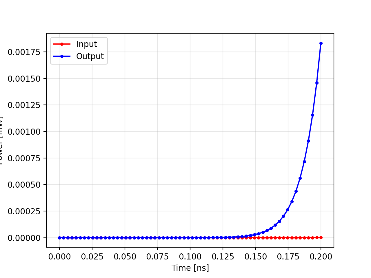
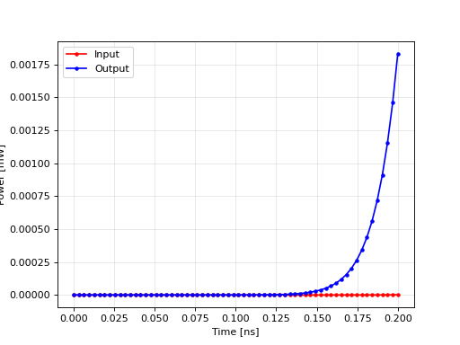
See the response of an optical fiber for a given input optical signal is very simple using
FIBER()device:
from opticomlib.devices import DAC, FIBER
from opticomlib import optical_signal, gv

gv(sps=32, R=10e9) # set again samples per slot and slot rate

P = 1e-3 # 1 mW of peak power

pulse_i = optical_signal(DAC('0001000', pulse_shape='gaussian', Vpp=P**0.5)) # create a gaussian pulse as before with (1 mW) of peak power and convert it as an optical_signal,
                                                                             # because of the FIBER device only accepts optical_signal as input

pulse_o = FIBER(pulse_i, length=100, alpha=0, beta_2=-20, beta_3=0, gamma=1.5) # propagate the pulse through a fiber of 100km length,
                                                                               # with alpha=0.2 dB/km, beta_2=-20 ps^2/km, beta_3=0 ps^3/km and gamma=1.5 1/W/km
                                                                               # see "Devices/FIBER" documentation page for more details of the FIBER device
pulse_i.plot('r.-', label='Input')
pulse_o.plot('b.-', label='Output').grid().legend().show()  # plot, grid, legend and show the input and output pulses
(Source code, png, hires.png, pdf)
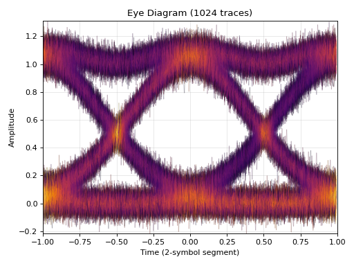
Estimate the eye diagram parameters and plot the eye of an arbitrary signal is very simple too, using
GET_EYE()device:
from opticomlib.devices import PRBS, DAC, gv, np

gv(sps=128, R=10e9) # set again samples per slot and slot rate

x = DAC(PRBS(order=15), pulse_shape='gaussian', Vpp=1) # create a PRBS signal and pass it through a gaussian pulse shaping filter with 1V output
x.noise = np.random.normal(0, 0.05, len(x)) # add gaussian noise to the signal

x.plot_eye(n_traces=1024, cmap='inferno', alpha=0.2)
x.show()
(Source code, png, hires.png, pdf)
